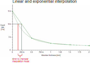
Problem descriptionWhen X-ray beam with continuous energy spectrum is used for transmission radiography, the beam hardening effect arises. Thicker i.e. more attenuating parts of the object attenuate softer parts of the original spectrum more effectively then thinner parts as illustrated in the next chart (measured with tungsten X-ray tube at 90kV and Medipix2 detector). |
||||||||||||||
 |
||||||||||||||
|
The X-ray beam energy spectrum varies from point to point behind an object of non-uniform attenuation. If efficiency of the sensor pixels is energy- dependent (and it is), then this effect leads to distortions whitch make tomographic reconstruction almost impossible. Moreover, if such an efficiency dependence is different for individual pixels, then even a single image is significantly distorted (see images below). |
||||||||||||||

 |
||||||||||||||
|
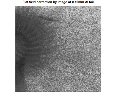
The flat field correction can improve the image distorted by non-uniform pixel efficiency, only for a certain absorber thickness. The pictures below show that the flat field correction using an open beam image will improve thin parts of the object, whereas the thick parts remain noisy. The situation is opposite to the flat field correction of the same data using an image of 0.16mm thick Aluminum foil. The thin parts are noisy while the thick ones are clear. |
||||||||||||||

 |
||||||||||||||
|
It is obvious that a certain level of flat field correction is necessary. This is achieved by an appropriate calibration method. The result is demonstrated in the following picture. All the object thicknesses are imaged without any noticeable noise. |
||||||||||||||
 |
||||||||||||||
|
As illustrated in the next chart, the efficiency of pixels differs significantly. The Beam Hardening (BH) plugin calibrates the efficiency of each individual pixel for curves corresponding to different attenuations. |
||||||||||||||
 |
||||||||||||||
|
It is necessary to prepare a set of perfectly flat calibrators of different thicknesses for correct calibration. The calibrators should cover the entire thickness range of the studied object. The calibrator material should be similar to the material of the object (in practice, this requirement is not absolute - Aluminum or plastic foils are suitable for most objects, incl. biological samples). The transmission measurement of each calibrator is required to obtain a set of calibration points for each pixel. X-ray tube settings and tube-detector distance must remain constant for all measurements. A complete set of calibration layers for each pixel is calculated as a function of the number of detected photons and the thickness of the calibration material. Interpolation is necessary between the calibration points. The Beam Hardening calibration plugin uses a "weighted exponential interpolation with offset" inside each interval. |
||||||||||||||
 |
||||||||||||||
|
It is possible to transform the measured data image (count rates) into equivalent absorber thicknesses using inversion of the calibration curve. For illustration, a calibration formula is shown below (y is count rate, yk is count rate in k-th calibration point, xkis thickness in k-th calibration point, ak is numerically precomputed parameter characterizing exponential base in k-th interval, and finally, c(y) is estimated object thickness): |
||||||||||||||
 |
||||||||||||||
|
The resulting image is dramatically improved, if the correct calibration curve for each pixel is used. Importantly, images are in the linear scale after the transformation. The linearization feature has a major impact on tomographic reconstruction methods. The transformation is superior to the standard flat-field correction, as it is valid for all ranges of attenuations and not only for a single value. Further details are described in this article. |
||||||||||||||
|
Operating BH correction plugin for
Pixelman
|
||||||||||||||
|
1) Prepare a set of calibrators covering the attenuation range of the object. For example, if the object ranges from 0 to 10 mm (biological) and your calibrators are made of plastic foils or wax, i.e. similar to the tissue, it is recommended to use thicknesses: 0, 0.1, 0.25, 0.5, 1, 2, 5, 10mm. The measurement of each calibrator should respect good statistics (e.g. 10 times higher then used for the object measurement). It is advisable to measure more points for low calibrator thicknesses, as the gradient of the curve is the highest at the starting point. |
||||||||||||||
|
|
||||||||||||||
|
|
||||||||||||||
|
|
||||||||||||||
|
|
||||||||||||||
|
|
||||||||||||||
Remarks and examples |
||||||||||||||
Preview of source data (not corrected):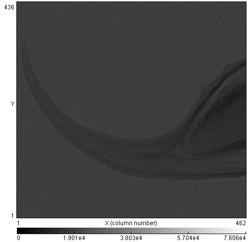 |
||||||||||||||
Preview of corrected Value (thickness): 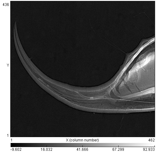 |
||||||||||||||
|
For additional information about pixels and calculation, select the "Advanced mode". It is accessible in "View -> Mode -> Advanced". The advanced information is shown at the bottom of the main window. Individual pixels can be selected by a left click on the image, after which four curves appear. The gray curve shows the median of the calibration points. This is masked by the overlying red curve showing weighted function calculated from the calibration points for certain pixels (red circles). The blue curves represent minimum and maximum value influenced by deviation. The black lines show the input count and the calculated thickness for the selected pixels. The yellow background indicates the actual deviation range. The advanced information window is divided into three sections. The first section from the left displays a table with coefficients for the selected pixel function. Each function is in the form " y = Aeax + P". The second section consists of the data used for calculations. The third one refer to calculated statistics displayed in the "Calculate info" panel in the right corner. The most important fields are the "Total", "Failed" and "OK". The calculated statistics does not depend on "Data". |
||||||||||||||
 |
||||||||||||||
Batch processing of imagesThe Plugin has a capacity to correct a set of measured objects as exemplified below. This shows a dialogue for processing a set of frames. It is accessible from the tools option in the main menu "Tools -> Batch processing of images..." item. The dialog consists of a left input section, that enable users to select the input frames, and a right output section. The input files are selected by filter "dsc" from the browse directory. The current setting generates two output files with names "[prefix]data R=181[suffix].txt" and "[prefix]data R=182[suffix].txt" into the same directory as the input directory. |
||||||||||||||
 |
||||||||||||||
Txt/Raw image translatorPlugin contains a file type translator. The dialog below is accessible from the main menu by "Tools->Raw/Txt Translator". This tool transforms file types: RAW->RAW, RAW->ASCII, ASCII->RAW and ASCII->ASCII. Conversion is possible for both single file (an image in the file) and multi file (set of images in the file). Transformation could change image range by formula: new_value = o + k * orig_value. If user requires same range of input/output files, the o = 0 and k = 1 should be set. Button "Check" check min/max range border of all selected files. |
||||||||||||||
|
|
||||||||||||||
Automatic calibration processCalibration points are measured automatically after you run the following steps. First, insert the calibrators into the revolver, then select the "Batch" option as a source, and finally click on the "Add" button. Wizard will guide you through a sequence of dialogs. The guide will calculate the estimated time, which can be either accepted or the settings can be changed. |
||||||||||||||
Plugin parametersPlugin parameters can be changed in "Mask & Interpolation", "Output Types" or "CPU setting" dialogs, which is accessible from main menu "Options -> Mask & Interpolation...", "Options -> Output Types..." and "Options -> CPU Setting...". You can restore default value of parameters by pressing the "Default" button.
|
||||||||||||||
 |
||||||||||||||
|
||||||||||||||
 |
||||||||||||||
|
||||||||||||||
 |
 2) Take several (e.g. 10) images of the first calibrator with good statistics (avoiding overflow of pixel counters), then open the main window of the Beam Hardening plugin (use tray menu) and press the "Add" button from the "Frames" source (for data stored on the disk select the "File" source). The Beam Hardening plugin will compute a sum of all frames in the Pixelman frame buffer and the standard deviation for each pixel. If just a single frame is measured, then a Poisson distribution is expected and the appropriate error is calculated. The total exposure time will be also obtained from the Pixelman. The first item named "(new item 0)" will appear in the list.
 3) Change the property of the item in the Edit box and confirm a new value by pressing the "Enter" key. Particular item can be selected by clicking on it. Repeat previous points for all prepared calibrators. You should not forget to specify the precise thickness for each of them!
  The "CALCULATE!" button will change the font to italic after the calculation of the calibration has finished. It means that no other calculation is necessary. The columns "bad", "median" and "deviation" will be changed for all calibration points in the table. The gray exponential function displayed in a plot below the table shows the relation between thickness and median of calibration points. The exponential function diagnostics will correct the dependence of the thicknesses and the medians.
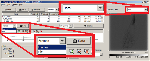 5) To increase the accuracy of the error estimation, measure the image several times. If just a single frame is measured, then a Poisson distribution is expected and the appropriate error is calculated. After you have finished the object measurements, select the source option "Frame" and press the "Data" button. To display the loaded data in the tight panel of the main windows, the "Data" option must be selected.
 6) To display results, select the "Corrected" option at the right corner of the main window. Image can be saved by pressing the right mouse button into image area (choose the option "Save image ..." or the "Copy to the clipboard"). Results are saved to ASCII files containing double values or picture formats JPG, PNG, GIF, TIFF, RAW. The Pixelman graphic transformation can be also applied on the results. The option "0.001-0.099 fractile" cuts all values under/over the fractile value. The BH calibration can be applied only after accomplished calculation process in the filter chain editor.